Key Takeaways
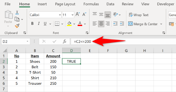
To use the less-than-or-equal-to operator, type “=C2<=200” where C2 is the cell to compare and 200 is your specified value. The formula will return TRUE if C2 has a value equal to or less than 200; else, it will return FALSE.
Using the less-than-or-equal-to
<=
operator in Microsoft Excel allows you to find out if the specified value matches your formula value or is less than that. We’ll show you how to use this operator to compare numbers and dates and how to use it with Excel’s various other functions.
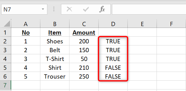
When you use the less-than-or-equal-to operator, Excel retrieves a TRUE result if the cell has a value that’s less than or equal to your specified value. If the cell value is higher than your specified value, the operator will return a FALSE result.
Use Less Than or Equal To for Numbers
If you want to find out whether a cell’s value is less than, equal to, or higher than your specified value, use the less-than-or-equal-to operator in your spreadsheet.
To do that, in your spreadsheet, select the cell where you want to display the result. In this cell, type the following formula and press Enter:
=C2<=200
In this formula:
-
C2refers to the cell whose value you want to check. -
200is your specified value. The formula will return aTRUEorFALSEresult based on this number.
And instantly, you’ll see the result in your selected cell. To copy the formula for all your records, from the bottom-right corner of the cell where you’ve entered the formula, drag downwards covering all your records.
And that’s all.
Use Less Than or Equal To for Dates
To find out if an event occurred before or on a specific date, use the less-than-or-equal-to operator along with Excel’s DATEVALUE function. The DATEVALUE function formats your data in a date format, so that the less-than-or-equal-to operator doesn’t retrieve the wrong result.
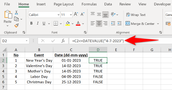
To use it, in your spreadsheet, click the cell where you want to see the formula result. In this cell, type the following formula and press Enter:
=C2<=DATEVALUE("4-7-2023")
In this formula:
-
C2refers to the cell where your date is given. -
DATEVALUEis the function that tells the formula that you’re using a date. -
4-7-2023(4 July 2023) is the date we’ve used in this example.
If your cell’s date falls on or before July 4th, 2023, then the formula will return a TRUE result. However, if your date falls after the 4th of July 2023, then you’ll get a FALSE result in your cell.
Feel free to use the above formula for any of your dates.
Use Less Than or Equal To With the IF Function
It makes more sense to use the less-than-or-equal-to operator along with an Excel function like IF than using it alone. With the IF function and based on your operator’s result, you can perform various actions in your spreadsheet.
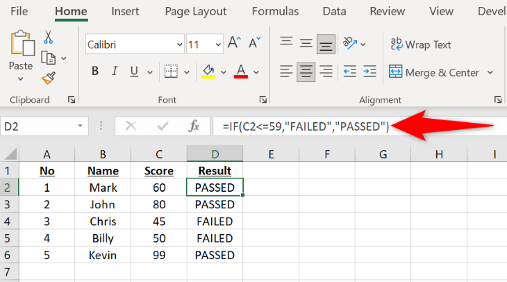
For example, if you’ve held an exam where anyone scoring 59 or less is to be marked FAILED and those getting a score of 60 or higher to be marked PASSED , use the less-than-or-equal-to operator with the IF function as follows:
=IF(C2<=59,"FAILED","PASSED")
In this formula:
-
C2refers to the cell where the score is displayed. -
59is the number that will be matched against the score. -
FAILEDis the message that will appear if someone has obtained59or less mark. -
PASSEDis the message that will be shown if someone has scored60or higher.
You’ll instantly see the result in your selected cell, and you’re all set.
Use Less Than or Equal To With SUMIF Function
By using the less-than-or-equal-to operator with Excel’s SUMIF function, you can sum only those numbers that match your criteria (i.e., equal to or fall below your specified number).
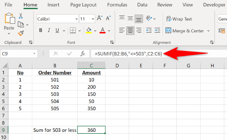
As an example, if you have a spreadsheet where you want to sum the order amounts only for the order numbers 503 or less, you’d use the following formula:
=SUMIF(B2:B6,"<=503",C2:C6)
Here:
-
B2:B6is the cell range where the function will apply your criteria. -
503is the number that will filter your data. -
C2:C6is the cell range whose amounts the function will sum if the given criteria matches.
And that’s it.
Use Less Than or Equal To With COUNTIF Function
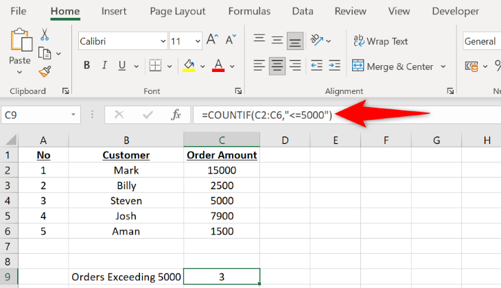
The COUNTIF function lets you count the number of cells that match your criteria. Here, you can use the less-than-or-equal-to operator to only count the cells having a value that either matches your given number or is less than that.
You’ll use it in your spreadsheet as follows:
=COUNTIF(C2:C6,"<=5000")
In this formula:
-
C2:C6is the cell range where your numbers are given. -
5000is your criteria. If a cell has a value of5000or less, it will be counted in your total number of cells.
You’re done.
And that’s how you use the less-than-or-equal-to operator in your Excel spreadsheets to perform your calculations. Enjoy!

